Table 2. FRECON3V mesh dependence test:
|
Run |
Mesh |
Umin |
Umax |
Wmin |
Wmax |
Nc |
|
FRE1 |
21x21 |
‑141.9 |
101.4 |
-225.6 |
215.2 |
7.05 |
|
FRE2 |
41x41 |
‑156.1 |
101.1 |
-177.0 |
213.1 |
6.98 |
|
FRE3 |
81x81 |
‑158.7 |
102.9 |
-175.7 |
217.3 |
6.60 |
|
FRE4 |
121x121 |
‑158.8 |
103.1 |
-175.8 |
221.4 |
6.52 |
|
FRE5 |
161x161 |
‑159.1 |
103.3 |
-175.9 |
222.0 |
6.49 |
|
FRE6 |
201x201 |
-159.2 |
103.3 |
-175.9 |
221.9 |
6.48 |
|
FRE7 |
301x301 |
-159.2 |
103.4 |
-176.0 |
222.5 |
6.47 |
|
Run |
Horizontal line
Y=0.5 |
Vertical line X=0.5 |
||||||
|
Umin/X |
Umax/X |
Wmin/X |
Wmax/X |
Umin/Y |
Umax/Y |
Wmin/Y |
Wmax/Y |
|
|
FRE1 |
-103.0/.80 |
20.4/.55 |
-211.0/.80 |
215.0/.05 |
-96.6/.15 |
82.0/.90 |
0.75/.95 |
9.72/.30 |
|
FRE2 |
-132.0/.72 |
6.25/.42 |
-174.0/.72 |
209.0/.05 |
-75.4/.25 |
84.2/.90 |
-68.9/.25 |
5.54/.60 |
|
FRE3 |
-131.0/.71 |
3.65/.39 |
-174.0/.71 |
213.0/.04 |
-76.8/.28 |
86.0/.89 |
-84.5/.26 |
6.28/.64 |
|
FRE4 |
-131.0/.71 |
3.21/.38 |
-175.0/.71 |
216.0/.04 |
-77.4/.28 |
86.5/.89 |
-86.6/.26 |
6.40/.65 |
|
FRE5 |
-131.0/.71 |
3.06/.38 |
-175.0/.70 |
216.0/.04 |
-77.6/.29 |
86.6/.89 |
-87.2/.26 |
6.44/.65 |
|
FRE6 |
-131.0/.71 |
3.00/.38 |
-175.0/.70 |
216.0/.04 |
-77.7/.29 |
86.6/.89 |
-87.5/.26 |
6.46/.65 |
|
FRE7 |
-131.0/.71 |
2.94/.38 |
-175.0/.70 |
217.0/.04 |
-77.8/.29 |
86.7/.89 |
-87.7/.26 |
6.48/.65 |
|
Run |
Mesh |
Umin |
Umax |
Wmin |
Wmax |
Nu |
|
FLU0 |
38x38 |
-158.94 |
105.31 |
-172.38 |
208.12 |
6.59 |
|
FLU1 |
76x76 |
-159.39 |
103.57 |
-173.61 |
220.60 |
6.47 |
|
FLU2 |
190x190 |
-159.77 |
103.51 |
-174.57 |
223.21 |
6.51 |
|
FLU3 |
380x380 |
-159.73 |
103.55 |
-174.73 |
223.52 |
6.50 |
|
Run |
Horizontal line
Y=0.5 |
Vertical line X=0.5 |
||||||
|
Umin/X |
Umax/X |
Wmin/X |
Wmax/X |
Umin/Y |
Umax/Y |
Wmin/Y |
Wmax/Y |
|
|
FLU0 |
-136.04/.71 | 2.46/.39 | -171.09/.71 | 202.15/.053 | -80.35/.29 | 88.92/.89 | -87.17/.26 | 6.25/.63 |
|
FLU1 |
-134.08/.71 | 2.83/.38 | -172.41/.71 | 215.36/.039 | -78.87/.29 | 87.18/.89 | -87.90/.26 | 6.39/.64 |
|
FLU2 |
-132.72/.71 | 2.92/.38 | -173.40/.70 | 217.53/.040 | -78.22/.28 | 86.90/.89 | -87.62/.26 | 6.44/.64 |
|
FLU3 |
-131.68/.70 | 2.93/.38 | -173.62/.70 | 217.84/.042 | -78.11/.28 | 86.85/.89 | -87.37/.26 | 6.42/.64 |
|
Run |
Elements |
Umin |
Umax |
Wmin |
Wmax |
Nu |
|
FID1 |
39x39 |
-155.10 |
104.30 |
-178.07 |
227.02 |
6.64 |
|
FID2 |
77x77 |
-159.03 |
105.38 |
-174.93 |
225.17 |
6.44 |
|
Run |
Horizontal line Y = 0.5 |
Vertical line X = 0.5 |
||||||
|
|
Umin/X |
Umax./X |
Wmin/X |
Wmax/X |
Umin/Y |
Umax./Y |
Wmin/Y |
Wmax/Y |
|
FID1 |
-130.47/.71 |
4.36/.39 |
-177.15/.71 |
218.50/.05 |
-77.05/.29 |
94.14/.92 |
-83.74/.26 |
6.03/.60 |
|
FID2 |
-131.50/.70 |
5.28/.38 |
-174.31/.70 |
219.71/.04 |
-81.60/.29 |
87.57/.89 |
-99.19/.26 |
7.19/.68 |
|
Run |
Mesh |
Umin |
Umax |
Wmin |
Wmax |
Nu |
|
STR1 |
50x50 |
-178.51 |
116.425 |
-191.450 |
248.063 |
6.63 |
|
STR2 |
100x100 |
-168.73 |
108.743 |
-183.605 |
237.538 |
6.78 |
|
STR3 |
150x150 |
-165.34 |
106.777 |
-180.327 |
232.612 |
6.73 |
|
STR4 |
200x200 |
-163.60 |
105.728 |
-179.554 |
229.670 |
6.67 |
|
STR5 |
250x250 |
-162.45 |
105.047 |
-177.356 |
227.635 |
6.65 |
|
Run |
Horizontal line Y = 0.5 |
Vertical line X = 0.5 |
||||||
|
|
Umin/X |
Umax./X |
Wmin/X |
Wmax/X |
Umin/Y |
Umax./Y |
Wmin/Y |
Wmax/Y |
|
STR1 |
-147.20/.67 |
1.15/.37 |
-191.45/.67 |
237.34/.04 |
-95.57/.31 |
96.26/.90 |
-119.59/.29 |
7.10/.67 |
|
STR2 |
-139.71/.71 |
2.43/.37 |
-183.04/.70 |
230.38/.04 |
-84.74/.28 |
90.93/.89 |
-95.47/.26 |
6.64/.64 |
|
STR3 |
-137.10/.70 |
2.61/.38 |
-179.69/.70 |
226.18/.04 |
-82.09/.28 |
89.38/.89 |
-91.34/.25 |
6.55/.64 |
|
STR4 |
-135.64/.71 |
2.68/.38 |
-177.74/.70 |
223.58/.04 |
-80.78/.28 |
88.54/.89 |
-89.75/.26 |
6.51/.64 |
|
STR5 |
-134.14/.71 |
2.44/.38 |
-176.64/.70 |
221.48/.04 |
-79.62/.28 |
87.96/.89 |
-87.31/.26 |
6.52/.64 |
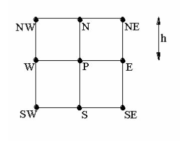
Figure 2.
Computational molecule
used in the diffuse approximation method
|
Run |
Number of Points |
Umin |
Umax |
Wmin |
Wmax |
Nc |
|
MEF1 |
10000 (100x100) |
-161.87 |
103.78 |
-167.58 |
225.94 |
6.22 |
|
Run |
Horizontal line Y = 0.5 |
Vertical line X = 0.5 |
||||||
|
|
Umin/X |
Umax./X |
Wmin/X |
Wmax/X |
Umin/Y |
Umax./Y |
Wmin/Y |
Wmax/Y |
|
MEF1 |
-125.34/.68 |
5.81/.34 |
-166.91/.64 |
218.89/.04 |
-79.87/.35 |
88.29/.89 |
-132.03/.31 |
6.56/.71 |
| Up | Down | Previous | Next |