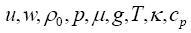
 denote respectively
the horizontal and the vertical velocity, the reference density of
fluid, the
pressure, the dynamic viscosity, the gravitational acceleration, the
temperature, the thermal condactivity and the specific heat. Water
physical properties, like
dynamic viscosity, specific heat, thermal conductivity and reference
density are assumed
constant and their value at the reference temperature Tref =
0oC are assumed. The values applied to the numerical models
are collected in Table 1.
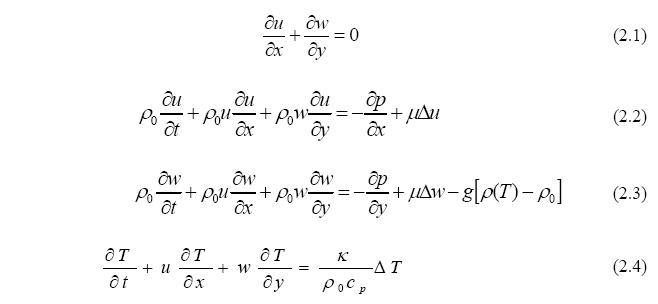
The anomalous thermal variation of the water density is implemented in
buoyancy
term only (eq. 2.3). The fourth order polynomial was used to describe variation of water density
with temperature:
denote respectively
the horizontal and the vertical velocity, the reference density of
fluid, the
pressure, the dynamic viscosity, the gravitational acceleration, the
temperature, the thermal condactivity and the specific heat. Water
physical properties, like
dynamic viscosity, specific heat, thermal conductivity and reference
density are assumed
constant and their value at the reference temperature Tref =
0oC are assumed. The values applied to the numerical models
are collected in Table 1.
The anomalous thermal variation of the water density is implemented in
buoyancy
term only (eq. 2.3). The fourth order polynomial was used to describe variation of water density
with temperature: 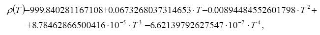
Table 1.
Physical properties of water used in the
simulations.
| Material properties of water at 0oC | Value | Unit |
|---|---|---|
 density of
water at
reference temperature density of
water at
reference temperature |
999.8 | kg/m3 |
 dynamic viscosity dynamic viscosity |
0.0017888 | kg/ms |
 thermal conductivity thermal conductivity |
0.566 | W/mK |
 specific heat specific heat |
4212.0 | J/kgK |
 gravitational acceleration gravitational acceleration |
9.81 | m/s2 |
 thermal expansion coefficient thermal expansion coefficient |
-6.733353E-05 | 1/K |
 , horizontal and vertical
coordinates X,Y, and
horizontal and
vertical velocities U,W the following
scales:
, horizontal and vertical
coordinates X,Y, and
horizontal and
vertical velocities U,W the following
scales: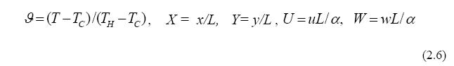
| Up | Down | Previous | Next |