I. Verification

4. Solution of numerical benchmark for thermal and viscous flows [7]

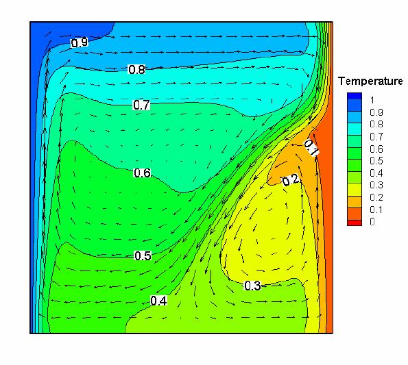
Figure 1 shows the velocity and temperature fields of obtained solution for defined problem. Two main circulations are clearly visible: an upper clockwise circulation transporting hot liquid towards the top wall and back along the isotherm of the density extremum, and a lower counter-clockwise circulation within the cold wall region. At the cold wall, the descending hot liquid interacts with the rising cold liquid. This creates a distinct saddle point in vicinity of the wall, approximately at about two-thirds of the cavity height. Position of the saddle point, given by the balance of competing positive and negative buoyancy forces, appears to be very sensitive to inaccuracies of the numerical solutions.

In order to compare performance of different codes in terms of their ability to reproduce fine details of the flow structure it is not sufficient to verify agreement of global flow field parameters, like those given in Tables 2-6. It appears that small deviation in their value (2% - 5%) from the reference solution, usually reported as reasonable or even excellent agreement, corresponds to distinct changes of the flow pattern. Such changes become responsible for differences in the local mass and heat transfer in the system. These effects can be perhaps neglected if only insulation or heat drainage are of the main interest. But they are not tolerable when phase change processes are present (e.g. freezing of water) or transport of small inclusions is an important issue. 

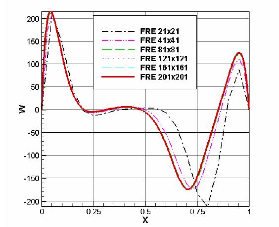
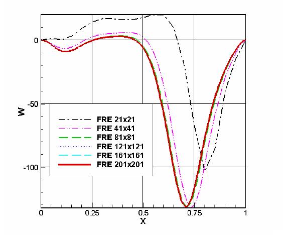
Hence, to obtain better insight into differences or similarities of the flow structures obtained from the investigated solvers, the second step of the verification procedure is proposed. It is based on calculating deviation of the velocity profiles extracted along three selected lines: horizontal centreline y=0.5, vertical centreline x=0.5 and vertical line passing through the mixing zone and the stagnation point at the cold wall (x=0.9). Locations of the lines are selected in such way that for any investigated mesh resolution they still match the nodes location, and additional interpolation errors are avoided. Figure 3 shows example of the velocity profiles along the horizontal and vertical symmetry lines of the cavity for meshes from Table 2. It is worth noting that the errors of the simulation performed for the quite fine mesh (FRE2) may reach almost 50% for the vertical velocity (Fig. 3a). Also large errors are present for the horizontal velocity component obtained for the coarse mesh (Fig. 3b). This test indicates that modelling of a simple natural convection in the presence of the strongly non-linear variation of water density requires careful analysis of results and very fine meshes.

 

The mesh sensitivity analysis performed for five investigated codes gives us some reference about convergence rate and allows to estimate their asymptotic behaviour. For more detailed comparison the flow field obtained using FRECON3V  for the fine mesh (201x201) was selected. The velocity and temperature profiles extracted along above mentioned lines are approximated with the high order polynomial and treated as a reference (benchmark) solution. The numerical values of the polynomials coefficients are given in Appendix. The fifteen digit accurate values of the coefficients are given to ease comparisons in the future. Obviously, it will be easier to quantify accuracy using well defined analytical functions than by overlapping reproduced figures.

An assessment on the accuracy of the solution is obtained calculating relative differences in terms of defined below standard deviations s, evaluated for the polynomials describing benchmark profiles and corresponding values extracted from the interrogated solution:

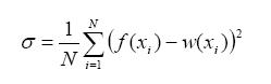
(4.1)

Here, N gives number of discrete points (corresponding to the discretization nodes) of the interrogates solution, w(x_i) polynomial value of the benchmark solution for the point x_{i ,} and f(x_i) value of the analyzed discrete solution for the point x_i.

Nine indicators are defined according to the above definition and used to evaluate accuracy of the solutions: σ_u1, σ_w1, σ_t1, σ_u2, σ_w2, σ_t2, σ_u3, σ_w3 and σ_t3.  They describe standard deviations calculated for two velocity components U ,W and temperature T for profiles extracted at centrelines Y=0.5,  X=0.5, and vertical line X=0.9.

The proposed accuracy indicators can be easily used to assess performance of any numerical solutions, regardless of dimension of the mesh size, as well as to estimate the rate of convergence of successive solutions. Data collected in Table 7 are presented in  Figure 4. The figures show, respectively, mesh dependence of σ _u1 , σ _w1 for velocity profiles at Y=0.5, σ _{u2 ,} σ _w2  for velocity profiles at X=0.5, σ _u3, σ _w3 for velocity profiles at X=0.9, and σ_{t1 ,} σ_t2,  σ _t3  for three temperature profiles at Y=0.5, X=05 and X=0.9.

The value of  σ _u1 , σ _w1  , σ _u2  σ _w2  , σ _u3, σ _{w3 ,} σ _{t1 ,}σ _{t2 ,}σ _t3 for the fine mesh FRECON solution (FRE6) was taken as a reference error indicator. Generously setting cut-off value for standard deviation equal 3 we come to conclusion that only solutions FRE4-7 and FLU3 are close enough to the reference solution to be assumed as the correct ones.  

From Figure 4 it is easily visible that the rate of convergence of SOLVSTR is much slower in comparison with FRECON. From the other hand, analysing the values of  the indicators on successive meshes we may find that the rate of convergence for FLUENT, FIDAP is almost linear in contrast to the much faster convergence of FRECON or even SOLVSTR. It is rather surprising as the both commercial codes claim to use second order approximations.

The stream function - vorticity solver SOLVSTR needs almost triple mesh refining (250x250) to reach accuracy comparable with that of other “mesh related” codes. One of the possible explanations of such behaviour is the lack of “upwind” schemes in SOLVSTR code. Moreover, improvement of the ADI algorithm and replacement of Gauss-Seidel algorithm by relaxation methods like SOR, CG, GMRES, could lead to better performance of the code.

It is worth noting that convergence of temperature is relatively easy to reach, and even for the most coarse meshes temperature profiles are practically “exact”. It indicates robustness of the energy equations and relatively small effect of the convective term on the resulting temperature distribution. It is rather surprising result, and it suggest that use of temperature as a convergence indicator can be dangerously misleading. At least for the analysed flow configuration.

A mesh-free code SOLVMEF using diffuse approximation fails this very sensitive test of accuracy. On the other hand the extremely long time of calculation does not allow for mesh refinement to increase the accuracy. Global and average indicators show proper trend of convergence. However, the main disadvantage of this method, its slow rate of convergence, is still challenging for future research.

 Figure 4. Mesh dependence: 

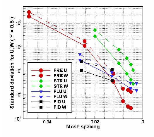
(a) – standard deviations σ _u1 , σ _w1 for velocity profiles at Y=0.5; 

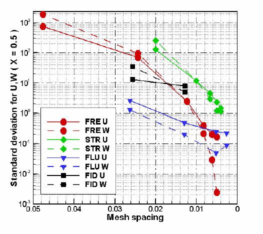
(b) - standard deviations σ _{u2 ,} σ _w2  for velocity profiles at X=0.5, 

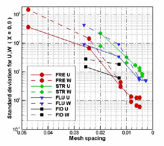
(c) - standard deviations σ _u3, σ _w3 for velocity profiles at X=0.9; 

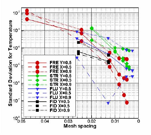
(d) - standard deviations σ_{t1 ,} σ_t2,  σ _t3  for three temperature profiles at Y=0.5, X=0.5 and X=0.9.