II. Validation
2. Definition of experimental benchmark
2.1. Experimental
set-up
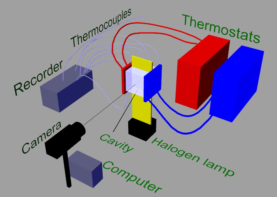
Figure 5 shows experimental set-up used in validation studies.
Figure 5 Sketch of experimetal set-up
Experimental set-up conists of :
- 3CCD colour camera XC003/P (Sony) with 32 bit module for image aquisition (Imaging Tech) (max. resolution 768x542 pixels)
- CMOS PCO 1200 hs black and white high speed camera (PCO Imaging)
with internal frame graber for image aquisition (max. resolution
1280x1024 pixels, maximum frame rate: 40720 fps)
- cavity
- halogen lamp (1000 Watt)
- two thermostats
- multi channel precision thermometer (PTM 3040 Prema Semicondutor GmbH)
- two PC computers
- set of thermocouples NiCr - NiAl of type K or Pt-100
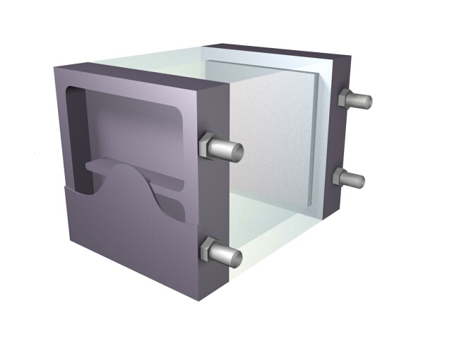
Figure 6 shows a cavity used in experiments. All dimenisons of the
cavity can be taken from files in Auto Cad format (*.dwg), which
present corss-sections of the cavity
files in *.dwg format : Central Vertical Cross-Section, Central Horizontal Cross-Section
files in *.jpeg format : Central Vertical Cross-Section, Central Horizontal Cross-Section
Figure 6 Sketch of the cavity
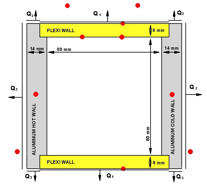
Figure 7 Central cross-section of the cavity with location of thermocoupes
2.2. Experimental
techniques
We made use of following experimental techniques:
Particle Image Velocimetry
Particle Image Velocimetry was used to obtain 2D velocity field for the
central cross-section of the cavity (Figure7). This method allows for
non-destructive and quantitative measurementd of velocity fields. The
first stage of the measurements include recoridng sequences of
images. Tracers are suspended uniformly inside the cavity. Two kind of
tracers were used in our measurements: thermocromic liquid crystals(see
details in next chapter) and pollens (Pinus silvestris, Pinus
nigra).
In the next stage, two subseqent flow images are analyzed with the use
of digital image techniques in order to obtain relative displacement of
tracers. Images ared divided into windows (sections) and for these
windows displacement is calculted on the basis of analysis of
correlation coeficients, FFT or others [XX,XX,XX].
Taking into account calculated relative displacement and time delay
between images velocity field is obtained for this pair of images. By
repeating this procedure for each of two subsequent digital images from
the recorded sequence, we were able to obtain series of velocity
fields. Then the average velocity field is calculated:
(X.X1)
Standard deviation for the whole velocity field is also analyzed in
order to determine the most appriopraite time delay between images:
(X.X2)
Precsision of average velocity fields was evaluted on the basis of mean dispersion of the average (X.X1), defined as follows:
(X.X3)
Triple maximum value of the mean disperison (X.X3) in the
whole velocity field was used as the quantitative measure of precision
for all velocity measurements making use of PIV.
Particle Image Thermometry
Particle Image Thermometry was used to obtain 2D temperature field for
the
central cross-section of the cavity (Figure7). This method allows for
non-destructive and quantitative measurementd of temperature fields.
The
first stage of the measurements include recoridng sequences of
colour images. As tracers the Thermochromic Liquid Crystals were
used, which were suspended uniformly inside the cavity. These tracers
reflect white halogen light only in the central cross-section of the
cavity (see Figure 5). Thermochromic liquid crystals change their
colour with temperature.
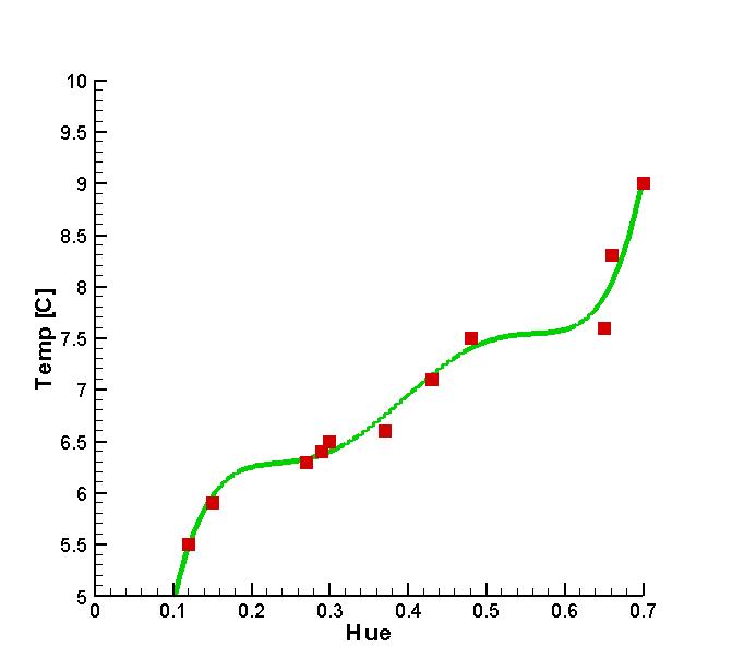
Colour images are analyzed making use of digital image
procedures. Temperature fields are obtained on the basis of
digital coulor images making use of calibration curves. Calibration
curve binds one of the component of digital image (H - Hue) with local
temperature. Form of this curve is determined in calibration process
for each of the Thermochromic Liquid Crystal applied.
Table 2.2.1. Thermochromic liquid crystals used in our researach
|
|
Symbol
|
Vendor
|
Initial temperature of sensitivity
|
Range of colour-play
|
|
1
|
BM100/R6C12W/S33
|
Hallcrest Ltd.
|
6 °C
|
12°C
|
|
2
|
TM445 (R17C6W)
|
BDH
|
17°C
|
6°C
|
|
3
|
TM317 (21C)
|
BDH
|
21°C
|
20°C
|
|
4
|
MixC (TM912+)
|
Merc
|
-2°C
|
10°C
|
|
5
|
TCC 1001
|
Merc
|
27°C
|
4°C
|
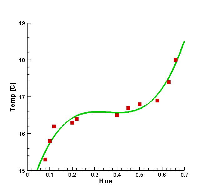
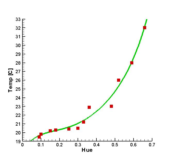
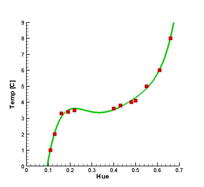
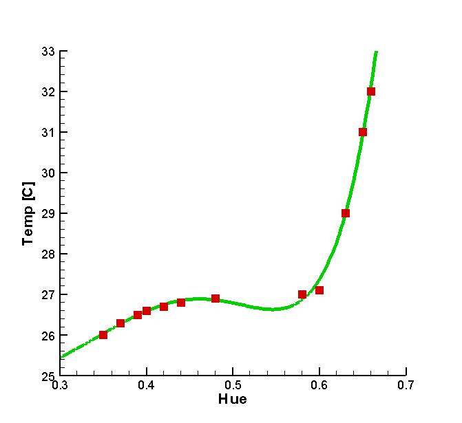
Calibration process was performed for each of TLCs from Table 2.2.1.
Calibration curves are presented below with analitical formula in form
of polynom.
Fiugre 8. Hallcrest
Figure 9. TM445
Figure 10 TM312
Figure 11 Mix C
Figure 12 TC1001
Point temperature measurements
High Speed Imaging - 2D Visualisation
2.3. Sensitivity
analysis